
The Poisson distribution, named after the French mathematician Siméon-Denis Poisson, is a fundamental tool in finance for modeling rare events such as credit defaults in a loan portfolio. It estimates the probability of observing a certain number of defaults over a given period.
In this article, we will explain the formula of the Poisson distribution, how modifying its parameters affects probabilities, and why it is essential in financial risk modeling.
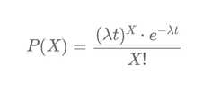
1. Understanding the formula
The probability of observing exactly X defaults over a period t, given an average default rate λ, is given by:
\[ P(X) = \frac{(λ t)^X \cdot e^{-λ t}}{X!} \]
where:
- λ represents the average number of defaults per year.
- t is the observation period in years.
- X is the number of observed defaults.
- e^{-λ t} represents the probability of observing no defaults.
- (λ t)^X weights the probability based on the expected number of defaults.
- X! normalizes the distribution to avoid multiple counting.
2. Effect of increasing λ (default rate) while keeping t and X constant
We increase λ, while keeping t = 1 and X = 1:
- λ = 1 → P(1) ≈ 36.79%
- λ = 2 → P(1) ≈ 27.07%
- λ = 5 → P(1) ≈ 3.37%
- λ = 10 → P(1) ≈ 0.045%
As λ increases, the probability of observing exactly one default drops sharply. A higher default rate makes multiple defaults more likely. The exponential decay (exp -λ * t) ensures that lower values become less probable.
3. Effect of increasing t (observation period) while keeping λ and X constant
We fix λ = 1 and X = 1, and increase t:
- t = 1 year → P(1) ≈ 36.79%
- t = 2 years → P(1) ≈ 27.07%
- t = 5 years → P(1) ≈ 3.37%
- t = 10 years → P(1) ≈ 0.045%
A longer observation period increases the likelihood of observing multiple defaults. The exponential decay (exp -λ * t) ensures that over time, observing only one event becomes very unlikely.
4. Effect of increasing X (number of defaults) while keeping λ and t constant
We fix λ = 1 and t = 1, and vary X:
- X = 1 → P(1) ≈ 36.79%
- X = 2 → P(2) ≈ 18.39%
- X = 5 → P(5) ≈ 0.31%
- X = 10 → P(10) ≈ 0.001%
Probability first rises, peaks near X ≈ λ t, then declines. The factorial term (X!) in the denominator grows much faster than the numerator, reducing the probability of extreme values.
5. Why does this matter for default risk modeling?
The Poisson distribution helps risk managers to:
- Predict the expected number of defaults over a given period.
- Assess extreme scenarios for stress testing.
- Model the distribution of defaults in a portfolio.
However, it has limitations:
- It assumes that defaults are independent, while in reality, they often correlate, especially during crises.
- It requires a constant default rate λ, whereas economic cycles influence this rate.
- It ignores contagion effects, where one default can trigger others.
- It does not account for structural portfolio adjustments, such as loan repayments or restructuring.
Despite these limitations, the Poisson distributionremains a powerful tool for quantifying risk exposure. Understanding its mechanics allows finance professionals to anticipate defaults, allocate capital efficiently, and manage credit risk effectively.
🎓 Formation recommandée : Les fondamentaux de la Finance Quantitative
Découvrez les concepts essentiels de la finance quantitative, explorez les modèles mathématiques appliqués et apprenez à les utiliser pour la gestion des risques et la valorisation des actifs.
Découvrir la formation
🎓 Formation recommandée : Mathématiques Financières - Niveau 2
Approfondissez vos connaissances en mathématiques financières, sachez identifier et utiliser les principales lois de probabilité utlisées dans la modélisation des marchés et dans la gestion des risques.
Découvrir la formation
Écrire commentaire