
The Vasicek Model, named after Oldřich Vašíček, is a fundamental mathematical framework used in finance to describe the evolution of interest rates over time. It is a type of stochastic differential equation (SDE) that belongs to the family of continuous-time models used specifically for interest rate modeling.
Key features of the Vasicek model include:
1. Mean Reversion: Like many interest rate models, the Vasicek model assumes that interest rates tend to revert to a long-term mean or equilibrium level over time. This feature captures the behavior of interest rates observed in real-world markets.
2. Volatility: The model incorporates volatility, allowing interest rates to vary stochastically. This accounts for the uncertainty and fluctuations commonly observed in interest rate data.
3. Speed of Mean Reversion: The Vasicek model includes a parameter that determines the speed at which interest rates revert to the mean. A higher speed of mean reversion implies faster convergence to the equilibrium interest rate.
Mathematically, the Vasicek model can be represented by the following stochastic differential equation:
\( dr(t) = \kappa(\theta - r(t)) dt + \sigma dW(t) \)
Where:
\( r(t) \): the short-term interest rate at time \( t \).
\( \kappa \): the speed of mean reversion.
\( \theta \): the long-term mean or equilibrium interest rate.
\( \sigma \): the volatility parameter.
\( dW(t) \): a Wiener process, representing randomness.
The Vasicek model is widely used in fixed-income markets and for pricing interest rate derivatives. It provides a structured way to model the stochastic evolution of interest rates over time.
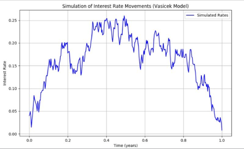
Example: Simulating Interest Rates Using the Vasicek Model
Given Parameters:
Long-term mean interest rate (\( \theta \)): 5%
Speed of mean reversion (\( \kappa \)): 0.1
Volatility (\( \sigma \)): 0.2
Initial interest rate (\( r(0) \)): 4%
Goal: Simulate the interest rate over one year using daily time steps.
Steps:
1. Define the time step (\( \Delta t \)) and the number of time steps (\( N \)): \( \Delta t = \frac{1}{365} \) (daily), \( N = 365 \) (one year).
2. Initialize \( r(0) = 0.04 \) and create an array to store interest rates.
3. Simulate interest rate changes iteratively using the Vasicek model:
\( r(t + \Delta t) = r(t) + \kappa(\theta - r(t)) \Delta t + \sigma \sqrt{\Delta t} Z \)
Here, \( Z \) is a random variable drawn from a standard normal distribution (\( Z \sim N(0, 1) \)).
4. Repeat for all \( N = 365 \) time steps to generate the full path of interest rates.
Detailed Example:
Let’s calculate the first three days step-by-step with example values for \( Z \):
- Day 1: Let \( Z = 0.5 \).
\( r(1) = 0.04 + 0.1(0.05 - 0.04)(1/365) + 0.2 \sqrt{1/365} \cdot 0.5 \)
\( r(1) \approx 0.04 + 0.00000274 + 0.002612 \)
\( r(1) \approx 0.04261 \) (or 4.261%). -
- Day 2: Let \( Z = -0.3 \).
\( r(2) = 0.04261 + 0.1(0.05 - 0.04261)(1/365) + 0.2 \sqrt{1/365} \cdot (-0.3) \)
\( r(2) \approx 0.04261 + 0.00000202 - 0.001566 \)
\( r(2) \approx 0.04105 \) (or 4.105%). -
- Day 3: Let \( Z = 0.8 \).
\( r(3) = 0.04105 + 0.1(0.05 - 0.04105)(1/365) + 0.2 \sqrt{1/365} \cdot 0.8 \)
\( r(3) \approx 0.04105 + 0.00000245 + 0.004177 \)
\( r(3) \approx 0.04523 \) (or 4.523%).
Repeat this process for all 365 days using new random values for \( Z \) at each step.
Simulated Results:
Sample output (example values):
Day 1: 4.261%
Day 2: 4.105%
Day 3: 4.523%
...
Day 365: 4.982%
The Vasicek model provides a powerful framework to simulate realistic interest rate paths over time. By incorporating mean reversion, volatility, and randomness, it models the behavior of interest rates in financial markets effectively.
Écrire commentaire