The variance of a Brownian motion in Simple Terms

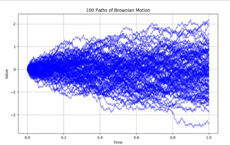
Brownian motion, a term often mentioned in the worlds of physics, mathematics, and finance, can be a puzzling concept to grasp. A seemingly random path that a particle traces in a liquid or gas medium, Brownian motion is often likened to the unpredictable movement of pollen particles in water. At its core, this stochastic process is governed by specific mathematical rules, one of the most intriguing being that its variance is directly proportional to time.

Before delving into its variance-time relationship, it's crucial to understand Brownian motion itself. Named after the botanist Robert Brown, who observed the erratic motion of pollen grains in water under a microscope, Brownian motion serves as a foundational model in stochastic calculus. Its most well-known application might be in the Black-Scholes model in finance, which aids in option pricing.

A standard Brownian motion, often symbolized as Wt, has a few defining properties:

• Starting Point: W0 = 0. This denotes that Brownian motion always begins at zero.
• Normal Distribution of Increments (*): For any two points in time s and t where s < t, the increment Wt - Ws follows a normal distribution. This distribution has a mean of 0 and, importantly for our discussion, a variance of t - s.

The intriguing characteristic of Brownian motion is the direct proportionality between its variance and time. In simpler terms, the randomness or spread of the Brownian motion's path increases as we observe it over a longer duration.

Imagine tracking the motion of a particle over intervals of 1 second and then 5 seconds. The unpredictability and potential paths the particle might take in 5 seconds vastly exceed those in the shorter 1-second window. The longer you watch, the more uncertain and spread out its position becomes. This growing uncertainty is mathematically captured by the variance increasing with time.

The time-dependent variance of Brownian motion has profound implications, especially in finance. When modeling stock prices or interest rates, the uncertainty or risk associated with longer time horizons becomes evident when using Brownian motion. For traders and investors, this can translate to increased potential rewards but also heightened risks.

(*) The term “increment” often refers to the change in a variable or a process over a specified time interval, especially in the context of stochastic processes. For example, the increment of a stock price between two different moments in time is simply the difference in its value at those two times.