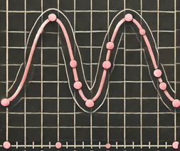
Runge’s phenomenon is a classic issue encountered in polynomial interpolation, particularly when high-degree polynomials are used to approximate a function over a given interval. Identified by Carl Runge in 1901, this phenomenon demonstrates that interpolation polynomials can exhibit significant oscillations, especially near the interval’s endpoints, diminishing the approximation’s quality. Consider the function f(x) = 1 / (1 + 25x²) defined on the interval [-1, 1]. Using evenly spaced interpolation points and a high-degree polynomial can lead to substantial oscillations, notably at the boundaries.
In quantitative finance, Runge’s phenomenon has notable implications in several applications:
Yield Curve Construction
When modeling an interest rate yield curve, available data often consist of discrete points corresponding to yields for specific maturities (e.g., 1 year, 2 years, 5 years, 10 years). Attempting to connect these points with a high-degree polynomial can induce significant oscillations, particularly at the maturity spectrum’s ends. For instance, a polynomial interpolating yields of 1%, 2%, 3%, and 4% might produce unrealistic rates (negative or excessively high) for maturities between or beyond these points.
Implied Volatility Surfaces
In finance, implied volatility surfaces (which relate volatilities to strike prices and maturities) are central to option pricing. The available data are often discrete, necessitating interpolation to construct a continuous surface. If this interpolation employs high-degree polynomials, oscillations from Runge’s phenomenon can introduce artifacts into the surface, such as unrealistic peaks or troughs, potentially leading to errors in pricing derivative products, especially exotic options.
Model Calibration and Stress Testing
During the calibration of financial models, like volatility models (Heston, SABR, etc.), parameters are adjusted to align with market data. If these data are affected by oscillations from improper interpolation, the calibration may yield biased results. Similarly, in stress testing scenarios, where interpolations simulate extreme conditions, unrealistic oscillations can distort conclusions.
Mitigating Runge’s Phenomenon
To prevent oscillations associated with this phenomenon, several approaches are favored in quantitative finance:
1. Piecewise Interpolation: A common method involves using cubic splines [1], which are polynomials defined piecewise between data points. These splines ensure smooth and continuous transitions without excessive oscillations.
2. Chebyshev Polynomials: Unlike uniformly spaced interpolation points, Chebyshev polynomials utilize optimal interpolation points, reducing oscillations. These points are concentrated near the interval’s ends, where oscillations typically intensify.
3. Non-Parametric Methods: Modern techniques like Gaussian processes or neural networks enable the construction of continuous approximations without directly relying on high-degree polynomials. These methods are particularly suited for complex surfaces, such as implied volatility surfaces.
4. Regularization: Introducing constraints or penalty terms in models can limit solution complexity and prevent excessive oscillations.
Illustrative Example
Suppose we aim to model a yield curve based on the following points:
- Maturities: 1 year, 3 years, 5 years, 10 years
- Yields: 2%, 2.5%, 3%, 3.5%
Using a third-degree polynomial to interpolate these points may cause the curve to oscillate significantly outside these points, potentially yielding rates near 1% or 5% for maturities slightly beyond the data range (such as 0.5 or 11 years). An alternative is to use a cubic spline, which provides a smoother and more realistic interpolation.
Runge’s phenomenon, though a theoretical concern, has practical implications in quantitative finance. Whether constructing yield curves, modeling implied volatility surfaces, or calibrating models, uncontrolled oscillations can lead to significant errors. By adopting appropriate techniques, such as cubic splines or non-parametric methods, it’s possible to develop robust and reliable approximations tailored to financial market needs.
[1] A cubic spline is an interpolation method that uses third-degree polynomials to connect successive data points in a continuous and smooth manner. Unlike global polynomial interpolation, which can result in unwanted oscillations (such as the Runge phenomenon), cubic splines divide the interval into segments, with each segment modeled by a distinct cubic polynomial. This approach ensures the continuity of the first and second derivatives at the junction points, thereby guaranteeing a seamless transition between segments. Cubic splines are widely used in quantitative finance to construct yield curves or volatility surfaces, as they offer increased flexibility while minimizing numerical artifacts.


Écrire commentaire