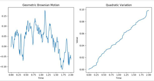
Brownian motion, a cornerstone concept in stochastic processes, illustrates a world of constant, random movement. Imagine a particle wandering unpredictably, with each step independent of the last. The resulting path is continuous yet non-differentiable at every point, making it one of the most intriguing phenomena in mathematics.
A continuous function is differentiable at a specific time
This unpredictability is encoded in the very definition of Brownian motion. If
This property, combined with its continuity, leads to the counterintuitive fact that the path of Brownian motion is non-differentiable everywhere. This non-differentiability is not a flaw but a feature that captures the essence of randomness.
The roughness of Brownian motion paths can be quantified using a concept called quadratic variation. Unlike classical measures that smooth out irregularities, quadratic variation embraces and
measures this roughness. For a Brownian motion
where
This linearity reflects the accumulation of randomness over time, with every increment adding to the overall variability of the path.
In financial modeling, the properties of Brownian motion find extensive applications, particularly in the study of asset prices. Geometric Brownian Motion (GBM), a popular model for stock prices,
extends Brownian motion by incorporating a drift component and a volatility term. The evolution of a stock price
where
The linear relationship between quadratic variation and time in Brownian motion translates into a measure of market uncertainty. In GBM, this property helps quantify volatility, a critical
parameter for pricing derivatives and assessing financial risk.
The non-differentiability of Brownian motion reminds us that while financial markets can be modeled mathematically, their intrinsic randomness and unpredictability remain ever-present. This characteristic is a driving force behind the development of sophisticated tools in quantitative finance.
1 Quadratic variation measures the cumulative squared increments of a stochastic process, offering a way to quantify its "roughness" over a given time interval.


Écrire commentaire