
In financial modeling, we often distinguish between "real-world" (or "physical") probabilities and "risk-neutral" probabilities. Real-world probabilities reflect the actual likelihood of events occurring in the market. In contrast, risk-neutral probabilities adjust these likelihoods to factor in market risk preferences and the time value of money, essentially showing the probabilities in a world where investors are indifferent to risk.
This risk-neutral measure, which can be complicated to grasp intuitively, is the building block of any derivative pricing and not only contingent claim derivatives like options and swaptions but also forward commitments like futures and forwards.
The Radon-Nikodym Derivative
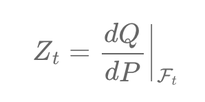
The Radon-Nikodym derivative serves as a crucial conversion tool. It adjusts the probabilities of future market behaviors from the real-world perspective to the risk-neutral one. Mathematically, if \( P \) represents the real-world measure and \( Q \) represents the risk-neutral measure, then the Radon-Nikodym derivative \( \frac{dQ}{dP} \) relates the two as:
where \( Z_t \) is a positive martingale adapted to the filtration \( \mathcal{F}_t \).
Girsanov's Theorem
However, it's not just about seeing differently; it's about recalibrating our models to these new views. This is where Girsanov's Theorem steps in, offering the mathematical levers to shift the drift of our financial processes accordingly.
If \( W_t \) is a Brownian motion under \( P \), Girsanov's Theorem states that under the new measure \( Q \):
where \( \theta_s \) represents the market price of risk and adjusts the drift.
Applications in Financial Models
This theorem ensures that once we've applied the Radon-Nikodym « conversion factor » to our models, they reflect a world where pricing is done without the possibility of arbitrage, ensuring fairness and consistency in the risk-neutral framework.
The HJM Framework
The HJM framework models the entire yield curve, or rather the forward rates, as opposed to just short rates. Girsanov's Theorem is used in this framework to ensure that the model is arbitrage-free by transforming the drift of forward rates under the real-world probability measure to the risk-neutral measure.
The CIR Model
The CIR model is a one-factor model of interest rate movements that assumes that the short rate follows a stochastic process:
Girsanov's Theorem is applied to switch the probability measure from the real-world to the risk-neutral, which is necessary for the pricing of zero-coupon bonds and other interest rate
derivatives.
The Hull-White Model
The Hull-White model is an extension of the Vasicek model, adding a time-dependent parameter to the drift term to fit the initial term structure of interest rates. It assumes:
Here, Girsanov's Theorem is used to derive an arbitrage-free model by adjusting the drift of the short-rate process when moving to a risk-neutral measure for derivative pricing.
In summary, Girsanov's Theorem provides the mathematical foundation to adjust stochastic processes from a real-world measure to a risk-neutral measure, which is a crucial step in the risk-neutral pricing of derivatives. The theorem ensures consistency, fairness, and arbitrage-free pricing, forming the backbone of modern financial mathematics.
Écrire commentaire