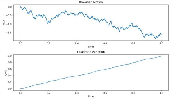
Imagine you're on a hiking trail. As you walk, the path goes up and down, sometimes smoothly and sometimes with sudden jolts. Now, if you're trying to describe how bumpy or smooth the trail is, you'll need a way to measure those ups and downs over your journey. The "quadratic variation" is a mathematical tool that helps measure this "bumpiness."
In the world of finance, instead of hiking trails, we have stock prices or other financial assets that move up and down over time.
To understand and predict these price movements, especially in a world where prices can change super quickly (like in high-frequency trading), traders and researchers use tools like the quadratic variation to get a sense of how volatile, or "bumpy," the price changes are.
Both quadratic variation and variance measure variability or "spread" in data. However, they are used in different contexts and have key differences:
- Variance: For a set of data points, you'd calculate the difference between each point and the mean, square it, and then take the average of those squared differences.
- Quadratic Variation: Instead of looking at the deviation from the mean, you're squaring the changes between consecutive data points and summing them up.
In the context of finance, Brownian motion (often termed as the Wiener process) is a mathematical model used to describe random movements over time, like the fluctuation of stock prices. Imagine a particle floating in a liquid and moving randomly. That's a real-world analogy of Brownian motion.
Now, if you were to look at the trajectory of this particle (or the fluctuation in stock prices) and try to measure its "bumpiness" or volatility, you'd use quadratic variation.
For a standard Brownian motion, W(t), over a time interval [0,T] its quadratic variation is simply T. This means that the sum of the squared changes like the stock price, as you divide the time interval into smaller and smaller pieces, approaches T.
This property is unique and crucial in distinguishing Brownian motion from other types of stochastic processes.
When modeling financial markets, particularly in the world of options pricing, the assumption is often that the change in asset prices follows a Brownian motion (plus some drift, giving rise to the Geometric Brownian Motion model). This is at the heart of the famous Black-Scholes option pricing model.
By understanding the quadratic variation of Brownian motion, financial mathematicians can make informed conclusions about the behavior, risk, and potential pricing of financial instruments.
In summary, quadratic variation helps measure the unpredictability or "bumpiness" of financial asset movements, which is crucial for traders and researchers to understand market behaviors.


Écrire commentaire