
Convexity plays a crucial role in market finance, particularly in pricing and valuing many financial instruments, such as bonds, whose price is affected nonlinearly by interest rate fluctuations, for options, where gamma measures the disproportionate impact of the underlying asset's price (like a stock) on its own price. From a mathematical perspective, a function is considered convex if its second derivative is positive. This characteristic implies that changes in one variable lead to nonlinear changes in another, which can offer benefits such as improved returns in finance.
Jensen's inequality
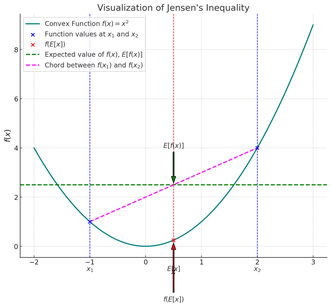
Jensen's inequality powerfully demonstrates convexity in mathematics. It connects the expected value of a convex function applied to a random variable to the function applied to the expected value of that variable. More precisely, Jensen’s inequality states that for any convex function \( f \) and any random variable \( X \), the following relationship holds:
This means that the expected value of the function \( f \) applied to \( X \) is at least as great as the function applied to the expected value of \( X \).
In financial terms, if a payoff function is convex, then the expected value of that payoff will be higher than the payoff calculated from the expected value of the underlying asset. This highlights the difference between the expectation of a financial derivative (with a convex payoff) and that of the underlying asset, which has major implications for financial products such as options.
Expected Value of the Function \( \mathbb{E}[f(X)] \)
The "expected value of the function," noted \( \mathbb{E}[f(X)] \), means that the function \( f \) is first applied to the random variable \( X \), and then its expectation is calculated. In other words, each possible outcome of \( X \) is evaluated through \( f \), and then a weighted average of all these values is computed.
Function of the Expected Value \( f(\mathbb{E}[X]) \)
The "function of the expected value," noted \( f(\mathbb{E}[X]) \), means that the expectation of the random variable \( X \) is first calculated, and then the function \( f \) is applied to this expectation. In other words, the average of all possible scenarios of the variable \( X \) is taken, and the function is then applied to this average.
Imagine a convex curve: if you draw a chord between two points on the curve (i.e., a straight line connecting them), the entire portion of the curve between these two points will lie below the chord. Similarly, if you calculate \( \mathbb{E}[f(X)] \), you take into account the whole convex curve, whereas \( f(\mathbb{E}[X]) \) only considers the central point (the average) and ignores the convexity of the curve.
The relationship between the convex curve and the chord reflects this idea: traversing the curve (which corresponds to \( \mathbb{E}[f(X)] \)) means "traveling more distance" or generating more returns than directly following the straight line (which corresponds to \( f(\mathbb{E}[X]) \)).
The convexity of the curve means that every fluctuation of the variable \( X \) is amplified in calculating the expected value. In finance, this results in higher returns, as the curve takes into account all positive variations of the underlying asset, unlike the chord, which ignores these fluctuations and represents just a simple average point.
Convexity of Interest Rate Products and Option Gamma
Convexity is a key concept for interest rate products (such as bonds) and options. For example, the convexity of interest rate products reflects the nonlinear way in which a bond’s price changes when interest rates fluctuate. The more convex a bond is, the greater its sensitivity to interest rate changes, allowing an investor to benefit asymmetrically from significant rate movements.
Similarly, for options, “gamma” represents the convexity of the option price concerning variations in the underlying asset. A high gamma means that delta (the sensitivity of the option price to the asset) changes quickly, causing a nonlinear reaction of the option price to changes. Thus, the option's convexity (via gamma) reflects its ability to benefit from extreme movements in the underlying asset.
Comparison with a Linear or Non Convex Curve (Futures and Forwards)
To understand convexity better, let's compare it to a linear function or to a financial product with a payoff that is neither convex nor concave, such as futures or forwards. These products have a linear (or quasilinear) relationship with the underlying asset. For example, a forward contract has a payoff that follows the underlying asset's variation proportionally: for every 1 unit change in the underlying price, the forward’s payoff changes by approximately 1 unit.
In contrast, for a financial instrument with a convex payoff (such as an option or a bond with positive convexity), the expected value of the payoff will be greater than that of the expected value of the underlying asset. This is because a convex curve amplifies the positive variations of the underlying asset while reducing the impact of negative variations.
Illustration
Let's take the example of a European call option. A call option has a convex gain curve: its payoff never drops below zero (if we exclude the premium paid to buy the option), and it increases in a growing manner once the underlying price exceeds the strike price.
Suppose a European call option on a stock XYZ with a strike price \( K \) of 100. If the stock price ends at \( S_1 = 120 \) or \( S_2 = 80 \), the option's payoff function is defined as:
Expected Gain of the Option: \( \mathbb{E}[f(X)] \)
If the stock ends at \( S_1 = 120 \), the gain is \( \max(120 - 100, 0) = 20 \). If the stock ends at \( S_2 = 80 \), the gain is \( \max(80 - 100, 0) = 0 \). The expected gain is:
Option Gain at the Expected Spot Price: \( f(\mathbb{E}[X]) \)
The expected value of the stock price is \((120 + 80)/2 = 100\). The gain of the option for this expected value is \( \max(100 - 100, 0) = 0 \).
Thus, Jensen’s inequality indicates that the expected gain of the option (10) is higher than the gain calculated from the expected spot price (0). This difference arises from the convexity of the
option's payoff, which amplifies potential gains during positive movements of the underlying asset.
Convexity amplifies potential gains during significant movements of the underlying asset, explaining the gap between the expected value of the payoff of a convex function (like an option) and that of a linear or nonconvex product like a forward.
Écrire commentaire