The Indicator Function Simply Explained

Indicator functions are crucial in financial mathematics, serving as binary conditions in the valuation of risky assets. They effectively act as switches in mathematical expressions, determining the inclusion or exclusion of certain terms based on the fulfillment of specific conditions.

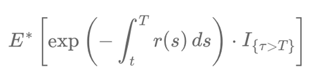
For instance, when assessing the value of a zero-coupon bond in a risk-neutral environment¹, we consider the expected present value of the payoff, discounted at the risk-free rate. The formula incorporates the indicator function to account for the possibility of issuer default. The valuation is expressed as:

\[ E^{\ast} \left[ \exp\left(-\int_t^T r(s) \, ds\right) \cdot I_{\{\tau > T\}} \right] \]

This formula assumes the payoff occurs only if the issuer does not default before the bond's maturity. The indicator function, \( I_{\{\tau > T\}} \), captures the event where the default time \( \tau \) occurs after the bond's maturity \( T \). Such modeling allows analysts to isolate scenarios where credit risk does not materialize, simplifying calculations under the risk-neutral measure.

Building on this concept, let's consider a more complex scenario where we introduce the possibility of default before maturity. The value of a risky zero-coupon bond is then given by the sum of two components – one reflecting the non-default scenario, and another accounting for the event of default. The formula for the valuation of a risky bond, considering the default risk, is:

\[ D(t, T) = E^{\ast} \left[ \exp\left(-\int_t^T r(s) \, ds\right) \cdot I_{\{\tau > T\}} + \exp\left(-\int_t^{\tau} r(s) \, ds\right) \cdot \delta \cdot I_{\{t < \tau \leq T\}} \right] \]

Here, the first term under the expectation represents the value if no default occurs, while the second term adjusts the value for the possibility of default before maturity, weighted by the recovery rate \( \delta \). This nuanced application of the indicator function allows financial analysts to model the complex dynamics of bonds where the risk of default is a significant factor.

Connecting to Quantitative Finance: Valuation Under Stochastic Models

The formulas above fit naturally into the framework of quantitative finance, where asset prices and interest rates evolve according to stochastic processes. In particular, the default event (\( \tau \)) is often modeled as the first jump time of a Poisson process or as the first passage time of a stochastic process crossing a boundary.

For example, under the reduced-form approach, the intensity of default is modeled using a Poisson process with intensity \( \lambda(t) \). The probability of default before time \( T \) is then:

\[ P(\tau \leq T) = 1 - \exp\left(-\int_t^T \lambda(s) ds\right) \]

In this case, the default intensity \( \lambda(t) \) may itself depend on macroeconomic factors, the firm’s credit rating, or even market signals like the price of credit default swaps (CDS).

Stochastic Interest Rates and the CIR Model

The formula for risky bond valuation also incorporates the evolution of interest rates via the term \( r(t) \), which can be modeled using the Cox-Ingersoll-Ross (CIR) process:

\[ dr(t) = \kappa (\theta - r(t)) dt + \sigma \sqrt{r(t)} dW(t) \]

Here:

- \( \kappa \): Speed of mean reversion.

- \( \theta \): Long-term mean of the interest rate.

- \( \sigma \): Volatility of interest rate changes.

- \( W(t) \): Standard Brownian motion representing market randomness.

By integrating this stochastic behavior into bond pricing models, we capture the uncertainty and dynamics of interest rates, which directly impact discount factors. Combining this with indicator functions allows analysts to build default-adjusted discount factors, accounting for both interest rate risk and credit risk simultaneously.

Applications in Pricing Derivatives and Structured Products

Beyond bond pricing, indicator functions play a vital role in pricing derivatives and structured products. For example, in credit default swaps (CDS), payouts depend on whether a credit event occurs before a specific date. This is modeled using indicator functions to define the payoff structure:

\[ CDS_{Payoff} = (1 - RR) \cdot I_{\{\tau \leq T\}} \]

Here, the recovery rate \( \delta \) and the probability of default (\( P(\tau \leq T) \)) determine the premium paid for the protection against default.

Balancing Arbitrage-Free Pricing with Risk Management

The integration of indicator functions into stochastic models ensures that pricing frameworks remain arbitrage-free. By modeling default risk, liquidity dynamics, and interest rate fluctuations, financial institutions can better manage risk exposure and design hedging strategies.

Furthermore, regulatory frameworks like Basel III emphasize the importance of stress testing such models under extreme conditions to ensure the resilience of financial systems.

¹ A risk-neutral environment assumes that there are no arbitrage opportunities, meaning that all assets are priced such that no risk-free profits can be made from market inefficiencies.