The Hessian in Finance Simply Explained

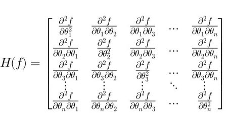
The Hessian in Finance Simply Explained

The Hessian matrix, a square matrix of second-order partial derivatives, is central to optimization and derivatives pricing. It plays a crucial role in determining the curvature of functions, which is essential in finance for portfolio optimization, risk management, and derivatives pricing. For a scalar function \( f(\theta_1, \theta_2, ..., \theta_n) \), the Hessian \( H \) is structured as:

\[ H(f) = \begin{bmatrix} \frac{\partial^2 f}{\partial \theta_1^2} & \frac{\partial^2 f}{\partial \theta_1 \partial \theta_2} & ... & \frac{\partial^2 f}{\partial \theta_1 \partial \theta_n} \\ \frac{\partial^2 f}{\partial \theta_2 \partial \theta_1} & \frac{\partial^2 f}{\partial \theta_2^2} & ... & \frac{\partial^2 f}{\partial \theta_2 \partial \theta_n} \\ ... \\ \frac{\partial^2 f}{\partial \theta_n \partial \theta_1} & \frac{\partial^2 f}{\partial \theta_n \partial \theta_2} & ... & \frac{\partial^2 f}{\partial \theta_n^2} \end{bmatrix} \]

This matrix captures not only the sensitivity of a function to changes in individual variables but also how changes in one variable influence another.

Optimization and Critical Points

In optimization, the Hessian classifies critical points by analyzing its eigenvalues (scalar values) and eigenvectors (direction vectors). For a Hessian matrix \( H \), an eigenvector is a non-zero vector \( v \) that, when multiplied by \( H \), changes only in magnitude: \( Hv = \lambda v \), where \( \lambda \) is the eigenvalue.

The eigenvalue \( \lambda \) quantifies how much the function curves along the eigenvector \( v \):

• \( \lambda > 0 \): The function curves upward (convex) along \( v \), indicating a local minimum.
• \( \lambda < 0 \): The function curves downward (concave) along \( v \), indicating a local maximum.
• \( \lambda = 0 \): No curvature (flat) along \( v \), suggesting a saddle point or an inflection point.

If all eigenvalues are positive, the function has a strict local minimum at that point. If some are positive and others are negative, the point is a saddle point, meaning that in some directions the function increases while in others it decreases.

Quadratic Approximation

The quadratic approximation near a point \( \theta_0 \) is:

\[ f(\theta) \approx f(\theta_0) + [\nabla f(\theta_0)]^T (\theta - \theta_0) + 0.5 (\theta - \theta_0)^T H(\theta_0) (\theta - \theta_0) \]

The term \( 0.5 (\theta - \theta_0)^T H(\theta - \theta_0) \) expands to a sum involving second derivatives, capturing interactions between variables. Eigenvalues of \( H \) determine whether this term grows (\( \lambda > 0 \)) or shrinks (\( \lambda < 0 \)) in specific directions.

In financial applications, this quadratic form helps approximate risk-return relationships in portfolio optimization and understand the curvature of profit functions.

Gamma Hedging

1. Univariate Case (Single Underlying \( S \))

For an option price \( V(S) \) dependent on a single underlying asset \( S \), the Gamma (\( \Gamma \)) measures convexity:

• \( \Gamma = \frac{\partial^2 V}{\partial S^2} \).
• \( \Gamma > 0 \): The option price exhibits positive convexity. This requires frequent adjustments to the Delta hedge (\( \partial V / \partial S \)) as \( S \) moves, as seen in vanilla options.
• \( \Gamma < 0 \): Less frequent but problematic, indicating negative convexity. Hedging becomes unstable, as seen in certain barrier options near knock-out levels.

2. Multivariate Case (Multiple Underlyings \( S_1, S_2, ..., S_n \))

For options dependent on multiple underlyings, the Hessian of the option price \( V \) generalizes Gamma to a matrix:

\[ H(V) = \begin{bmatrix} \frac{\partial^2 V}{\partial S_1^2} & \frac{\partial^2 V}{\partial S_1 \partial S_2} & ... & \frac{\partial^2 V}{\partial S_1 \partial S_n} \\ \frac{\partial^2 V}{\partial S_2 \partial S_1} & \frac{\partial^2 V}{\partial S_2^2} & ... & \frac{\partial^2 V}{\partial S_2 \partial S_n} \\ ... \\ \frac{\partial^2 V}{\partial S_n \partial S_1} & \frac{\partial^2 V}{\partial S_n \partial S_2} & ... & \frac{\partial^2 V}{\partial S_n^2} \end{bmatrix} \]

Eigenvalues of \( H(V) \) determine the convexity or concavity of the option price along specific directions (eigenvectors). When all eigenvalues are positive, hedging strategies are more predictable. When mixed eigenvalues occur, hedging becomes more complex and requires multi-dimensional strategies.

Uniform Convexity (all \( \lambda > 0 \)) : Simplifies hedging, as prices curve upward in all asset combinations.

Mixed Eigenvalues : Require multi-directional hedging to manage variations in risk exposure.