The Gumbel copula simply explained

A copula is a mathematical concept used in statistics to describe the relationship between multiple variables. Its main function is to capture the dependence structure between these variables, separate from their individual distributions.

In multivariate analysis, you often deal with multiple variables, each with its own distribution (margins). A copula allows you to study and model how these variables are related (dependence) independently from their individual distributions.

Essentially, a copula takes the individual distributions of variables and merges them into a joint multivariate distribution. This joint distribution reflects not just the individual behaviors of each variable but also how they interact or depend on each other.

Copulas work by using the cumulative distribution functions (CDFs) of variables, which are transformed to uniform distributions on the interval [0, 1].

After transforming the margins to uniform distributions, the copula then models the dependence structure between these variables. It essentially « ties» together the separate uniform distributions, creating a multivariate distribution that reflects the dependencies.

The Gumbel copula is a member of the Archimedean family of copulas. It's particularly well-suited for modeling tail dependencies, especially for variables that tend to show extreme values simultaneously.

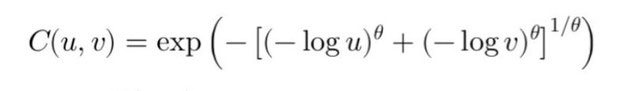
The Gumbel copula C(u, v) is defined using the formula: C(u, v) = exp(-[ (-log u)^θ + (-log v)^θ ]^(1/θ)) where u and v are the cumulative distribution functions (CDFs) of the variables, and θ is a parameter that controls the strength of the dependence, with θ ≥ 1.

Higher values of θ indicate stronger tail dependence.

Consider two financial assets, A and B, which are part of a CDO. We are interested in understanding the risk of joint defaults.

Assume that we have historical default data for these assets. Let's say the probabilities of default (within a year) for assets A and B are 5% and 10%, respectively.

For this example, we'll choose a θ value greater than 1 to reflect dependence, say θ = 2. This indicates a stronger dependency, especially in the tails.

First, we transform the default probabilities to uniform distributions. For simplicity, let's use the default probabilities directly as our uniform values. So, u (for asset A) = 0.05, and v (for asset B) = 0.10.

Plugging in the values:
u = 0.05, v = 0.10, and θ = 2.
We calculate (-log(0.05))^2, (-log(0.10))^2, and then add these values.
Raise the sum to the power of 1/2 (since θ = 2), and finally apply the exponential function.

The joint probability of both assets A and B defaulting simultaneously within the year, under our assumptions, is approximately 2.29%.

In the context of pricing CDOs in 2008, using such a model which emphasizes tail dependencies (like the Gumbel copula) could have provided a more realistic assessment of risk compared to Gaussian copulas.

hashtag#GumbelCopula