The Finite Difference Method in Simple Terms

One way to think about finite difference methods is by imagining a hike up a mountain trail. Suppose you take a big step forward, then look back to measure how much higher or lower you are compared to where you started. The difference in height over the distance of your step gives you an idea of the slope at that point.

Now, let's say you want a more accurate idea of the steepness right where you're standing. Instead of taking a big step, you take a very tiny step. The tinier the step, the more accurate your measurement of the slope at that exact point.

Finite Difference Methods

Finite difference methods are analogous to this hiking analogy. They measure how much a function (like the mountain trail) changes as you make tiny "steps" in the variable of interest (like your position on the trail). The smaller the step, the more accurate the measurement—but this also means more steps are needed to cover the whole trail!

These methods are used to approximate changes in various fields, whether it's the steepness of a curve, the temperature in a material, or the price of a financial option.

Application in Options Pricing

In options pricing, one of the key components we are interested in is how the price of an option changes as the price of the underlying asset (e.g., a stock) changes. This change rate is known as the "delta" of the option.

Imagine the mountain trail represents the option price, and each step represents a small change in the stock price. As you move along the trail (as the stock price changes), the steepness of the trail represents the delta. When taking tiny steps on the trail to determine steepness, you're essentially using the finite difference method to approximate the delta of the option.

Delta and Gamma: Measuring Changes in Changes

But just like on a mountain trail, the landscape of options isn't flat. The steepness (delta) itself can change. This "change of the change," or the rate at which delta changes, is known as "gamma."

Think about taking another set of steps and seeing how the steepness changes between those steps. In this case, you're approximating gamma using finite differences.

Real-World Options Pricing

In real-world options pricing:

• Delta: Answers the question, "If the stock price goes up by 1, how much will my option price change?"
• Gamma: Answers the question, "If the stock price goes up by 1 again, how will the change rate (delta) itself change?"

Mathematical Representation

To approximate delta using finite differences, we calculate:

\[ \Delta = \frac{V(S + h) - V(S)}{h} \]

Where:

• \( V(S) \): The option price at stock price \( S \).
• \( h \): A small step in the stock price.

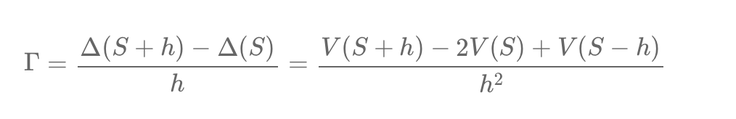
Similarly, to approximate gamma, we use:

\[ \Gamma = \frac{\Delta(S + h) - \Delta(S)}{h} = \frac{V(S + h) - 2V(S) + V(S - h)}{h^2} \]

These approximations allow us to understand the sensitivities of an option's price without needing the exact pricing formula.

Benefits of Finite Difference Methods

• Accuracy: Provides a detailed approximation of changes in option prices and their sensitivities.
• Flexibility: Can be applied even when the exact pricing formula is unknown.
• Widely Used: Essential in numerical simulations for complex derivatives and risk management.

Finite difference methods in finance are akin to taking tiny steps to understand the steepness of a trail. By approximating changes in option prices (delta) and changes in delta (gamma), these methods provide valuable insights into the dynamics of options pricing, enabling professionals to make more informed decisions.