
The trigonometric circle naturally extends the concept of complex numbers, using the unit circle as a framework to illustrate periodic phenomena. The binomial model in option pricing involves a financial derivative's price evolving over time in a binomial tree, reflecting market uncertainty. By analyzing future payoffs' expected value under a risk-neutral measure, the problem can be expressed using Fourier transforms. The characteristic function of the underlying asset's distribution is crucial, encoding key information about its behavior.
The link between binomial pricing models and Fourier transforms becomes even more apparent when we consider circular convolutions. Circular convolution is a mathematical operation that combines two sequences by convolving them in a circular manner, where the end of one sequence wraps around to the beginning.1
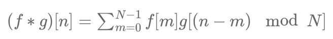
Mathematically, circular convolution can be expressed as:
\( (f * g)[n] = \sum_{m=0}^{N-1} f[m] g[(n - m) \mod N] \)
where \( f \) and \( g \) are sequences, \( N \) is the length of the sequences, and \( \mod N \) ensures periodic wrapping. This formula allows calculations to be performed efficiently using the Fast Fourier Transform (FFT).
In a multi-period framework, the binomial tree approach can become time-consuming due to the exponential growth in the number of nodes as the number of periods increases.
Instead of explicitly constructing and traversing the entire binomial tree, circular convolution allows us to compute the option prices at each time step by convolving the option payoffs with the state price matrix. This convolution operation involves a fixed number of multiplications and additions, regardless of the number of periods.
Let's consider a simplified example where we have a two-period binomial option pricing model with a risk-neutral probability of 0.6 for an up move and 0.4 for a down move. We'll visualize this scenario with the outer circle representing these probabilities and the inner circle containing different option payoffs.
Outer Circle (Adjusted Probabilities):
- Risk-neutral probability of 0.6 (up move) at 0 degrees.
- Risk-neutral probability of 0.4 (down move) at 180 degrees.
Inner Circle (Option Payoffs):
- Option payoff of $100 at 0 degrees.
- Option payoff of $150 at 90 degrees.
- Option payoff of $200 at 180 degrees.
Rotate the inner circle clockwise by one position, corresponding to one time step. For example, the $200 payoff moves to 270 degrees. Perform circular convolution by multiplying each option payoff with the corresponding probability at the same angle on the outer circle and summing up the results.
\( P(t+1) = \sum_{k=0}^{N-1} P_k(t) \cdot p_k \)
where \( P(t+1) \) represents the updated price, \( P_k(t) \) the payoff at time \( t \) for state \( k \), and \( p_k \) the probability weight.
Repeat this process for each time step to compute the expected payoffs iteratively.
1. Convolution: from "convolvere", roll together.
Inspiration from: Introduction To Fast Fourier Transform In Finance by Ales Cerny.
Écrire commentaire