
The Cox-Ingersoll-Ross (CIR) model is a fundamental tool in quantitative finance, widely used to model the dynamics of short-term interest rates. It addresses key challenges in interest rate modeling, such as mean reversion and the need to prevent negative interest rates. Developed in the early 1980s, the CIR model is expressed as a stochastic differential equation (SDE), capturing the random evolution of interest rates over time.
Key Features of the CIR Model:
The CIR model is defined by three primary characteristics:
- Mean Reversion: Interest rates tend to revert to a long-term mean or equilibrium rate \( \theta \). This feature aligns with economic theory, which suggests that interest rates fluctuate around an equilibrium driven by macroeconomic factors.
- Stochastic Volatility: The CIR model incorporates stochastic volatility, allowing the rate of change of interest rates to vary over time. This captures observed market behaviors, such as periods of high or low volatility in interest rates.
- Non-Negativity: The square-root diffusion term ensures that interest rates remain non-negative, an essential property for practical applications in finance.
Mathematical Representation
The dynamics of the short-term interest rate \( r(t) \) in the CIR model are governed by the following stochastic differential equation:
\[ dr(t) = \kappa(\theta - r(t))dt + \sigma\sqrt{r(t)}dW(t) \]
Where:
- \( r(t) \): The short-term interest rate at time \( t \).
- \( \kappa \): The mean reversion speed, controlling how quickly \( r(t) \) reverts to \( \theta \).
- \( \theta \): The long-term mean interest rate.
- \( \sigma \): The volatility parameter, determining the magnitude of randomness in \( r(t) \).
- \( dW(t) \): A Wiener process, modeling the stochastic component of \( r(t) \).
The drift term \( \kappa(\theta - r(t))dt \) represents the deterministic force pulling \( r(t) \) toward the mean \( \theta \). The diffusion term \( \sigma\sqrt{r(t)}dW(t) \) introduces randomness, with its magnitude dependent on \( \sqrt{r(t)} \). This dependency prevents \( r(t) \) from becoming negative.
Analytical Properties
The CIR model belongs to the family of affine term structure models, characterized by interest rate dynamics where bond prices can be expressed as exponential functions of affine forms in \( r(t) \). The CIR model has a closed-form solution for zero-coupon bond prices, making it highly practical in finance.
\[ P(t, T) = \exp(A(t, T) - B(t, T)r(t)) \]
Where \( P(t, T) \) is the price of a zero-coupon bond maturing at \( T \), and \( A(t, T) \) and \( B(t, T) \) are functions of model parameters, derived from solving a Riccati equation.1
Applications of the CIR Model:
The CIR model is widely applied in:
- Fixed Income Pricing: It is used to value bonds and other fixed-income securities by modeling the dynamics of short-term interest rates.
- Options on Interest Rates: The model aids in pricing options on bonds and interest rate derivatives, such as caps and floors.
- Credit Risk Models: The CIR process is often employed to model default intensity in credit risk frameworks.
Simulation of Interest Rates
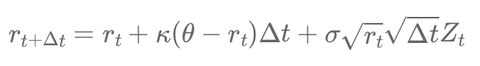
To simulate interest rates under the CIR model, the following discrete approximation can be used:
\[ r_{t+\Delta t} = r_t + \kappa(\theta - r_t)\Delta t + \sigma\sqrt{r_t}\sqrt{\Delta t}Z_t \]
Where \( Z_t \sim \mathcal{N}(0, 1) \) is a standard normal random variable, and \( \Delta t \) is the time step size.
Example: Simulating CIR Dynamics
Consider the following parameter values:
- Mean reversion speed (\( \kappa \)): 0.2
- Long-term mean (\( \theta \)): 0.05 (5%)
- Volatility (\( \sigma \)): 0.01
- Initial rate (\( r(0) \)): 0.03 (3%)
- Simulation horizon: 1 year
- Time step size (\( \Delta t \)): 1/252 (daily steps)
The simulation involves:
- Initial setting: \( r(0) = 0.03 \).
- For each step \( t \), generate a random number \( Z_t \sim \mathcal{N}(0, 1) \).
- Update \( r_t \) using the discrete approximation:
\[ r_{t+\Delta t} = r_t + \kappa(\theta - r_t)\Delta t + \sigma\sqrt{r_t}\sqrt{\Delta t}Z_t \]
Simulated interest rates will demonstrate mean reversion toward \( \theta \), with stochastic volatility reflecting market behavior.
The CIR model is a cornerstone in financial modeling. Its mean reversion property, non-negativity constraint, and analytical tractability make it an invaluable tool for interest rate and credit risk modeling. While the CIR model has limitations—such as a rigid volatility structure—it remains a benchmark model and a starting point for more sophisticated frameworks.
1 The Riccati equation is a type of differential equation widely used in finance for modeling dynamic systems, particularly in the pricing of bonds and derivatives.
Écrire commentaire