The Cholesky Decomposition in Simple Terms

Imagine you're trying to build a toy house using LEGO blocks. The stability of this house depends on the blocks and their arrangement. If you were to build a solid base using the right pieces, the entire house would stand firm. If not, it might wobble or even collapse.

Now, think of financial data like a big matrix (just a table of numbers). This matrix might contain information about various assets' returns, risks, and their interrelationships. Just like our LEGO house, we want to understand the structure of this data—specifically, how different assets interact with each other in terms of risk.

Enter the Cholesky decomposition! It's like taking our LEGO house apart to see the individual blocks and understand how they fit together. By applying this technique to our matrix, we can split our data into simpler components, making it easier to see the individual risk factors and how they relate to one another.

In quantitative finance, this can help professionals understand correlations between assets, model portfolio risks more accurately, and optimize investment strategies. By breaking complex data down into simpler parts, they can make more informed decisions and, hopefully, build a more stable financial "house."

So, in essence, Cholesky decomposition in quantitative finance is like using a special technique to see the building blocks of financial risk and understanding how they all fit together!

Continuing from our LEGO analogy: In the world of finance, much like in building LEGO structures, we're dealing with interconnected pieces. These pieces are assets in our portfolio, and they don't exist in isolation. Their returns are influenced by numerous factors like economic conditions, market sentiment, and global events. It's essential to understand these interconnections to make sound investment decisions.

Cholesky decomposition is one such technique used in these models. By understanding the core building blocks of these relationships, we can better anticipate how different events or conditions will impact the entire portfolio.

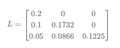
Imagine you have a portfolio of three assets: Stocks A, B, and C. You want to understand the correlation between these stocks to evaluate your portfolio’s risk. The covariance matrix (a mathematical representation of how these assets vary with respect to each other) of the returns of these stocks is provided. We can use the Cholesky decomposition to “decompose” this covariance matrix and understand the underlying relationships.

This decomposition can be further used in Monte Carlo simulations and other financial models to generate correlated asset paths or to simulate correlated asset returns. It’s particularly valuable in scenarios where we need to preserve the relationship (correlation) between different assets when generating random scenarios for simulations.