
Step 1: Constructing the Hedging Portfolio
We define the hedging portfolio \( \Pi \) as:
\( \Pi = V(S, t) - \Delta S \) (equation 1)
Where \( V(S, t) \) is the value of the call option as a function of the stock price \( S \) and time \( t \), and \( \Delta \) is the number of shares held in the portfolio.
The instantaneous change in the portfolio value is given by:
\( d\Pi = dV - \Delta dS \) (equation 2)
Step 3: Stock Price Dynamics
The stock price follows a stochastic process described by:
\( dS = \mu S dt + \sigma S dW \) (equation 3)
- \( \mu S dt \): Drift term, representing the deterministic component of the stock's return.
- \( \sigma S dW \): Diffusion term, capturing the random fluctuations in the stock price, where \( W \) is Brownian motion.
Using Itô's Lemma , the differential of the option value \( V \) is given by:
\( dV = \frac{\partial V}{\partial t} dt + \frac{\partial V}{\partial S} dS + \frac{1}{2} \frac{\partial^2 V}{\partial S^2} (dS)^2 \) (equation 4)
- \( \frac{\partial V}{\partial t} \): Theta, the rate of change of \( V \) with respect to time.
- \( \frac{\partial V}{\partial S} \): Delta, the sensitivity of \( V \) to changes in \( S \).
- \( \frac{\partial^2 V}{\partial S^2} \): Gamma, the convexity of \( V \) with respect to \( S \).
Substituting \( dS \) from equation (3) into \( (dS)^2 \), we find:
\( (dS)^2 = (\mu S dt + \sigma S dW)^2 \)
Simplifying using stochastic calculus rules :
- \( (\mu S dt)^2 = 0 \), since \( (dt)^2 = 0 \).
- \( 2(\mu S dt)(\sigma S dW) = 0 \), since \( dt \cdot dW = 0 \).
- \( (\sigma S dW)^2 = \sigma^2 S^2 dt \), using \( (dW)^2 = dt \).
Thus, the result is:
\( (dS)^2 = \sigma^2 S^2 dt \) (equation 5)
Using equation (5), the differential of \( V \) becomes:
\( dV = \frac{\partial V}{\partial t} dt + \frac{\partial V}{\partial S} dS + \frac{1}{2} \sigma^2 S^2 \frac{\partial^2 V}{\partial S^2} dt \) (equation 6)
Substituting \( dV \) from equation (6) into equation (2), we have:
\( d\Pi = \left( \frac{\partial V}{\partial t} + \frac{1}{2} \sigma^2 S^2 \frac{\partial^2 V}{\partial S^2} \right) dt + \left( \frac{\partial V}{\partial S} - \Delta \right) dS \)
Setting \( \Delta = \frac{\partial V}{\partial S} \) ensures that the stochastic term \( \left( \frac{\partial V}{\partial S} - \Delta \right) dS \) vanishes, leaving:
\( d\Pi = \left( \frac{\partial V}{\partial t} + \frac{1}{2} \sigma^2 S^2 \frac{\partial^2 V}{\partial S^2} \right) dt \) (equation 7)
Since the portfolio is risk-free, its change must equal the risk-free rate:
\( d\Pi = r \Pi dt \)
Substituting \( \Pi = V - \Delta S \) and \( \Delta = \frac{\partial V}{\partial S} \):
\( \frac{\partial V}{\partial t} + \frac{1}{2} \sigma^2 S^2 \frac{\partial^2 V}{\partial S^2} = r V - r S \frac{\partial V}{\partial S} \)
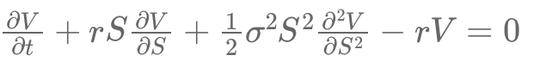
Rearranging terms, we obtain the Black-Scholes PDE:
\( \frac{\partial V}{\partial t} + r S \frac{\partial V}{\partial S} + \frac{1}{2} \sigma^2 S^2 \frac{\partial^2 V}{\partial S^2} - r V = 0 \)
In this equation, we identify key terms:
- \( \frac{\partial V}{\partial t} \): This represents the time value of the option, showing how the option's value decreases as it approaches maturity.
- \( r S \frac{\partial V}{\partial S} \): This term corresponds to the sensitivity of the option to the stock price (Delta) adjusted by the risk-free rate.
- \( \frac{1}{2} \sigma^2 S^2 \frac{\partial^2 V}{\partial S^2} \): This captures the impact of volatility and convexity (Gamma) on the option's value.
- \( -r V \): This accounts for the discounting effect at the risk-free rate.
🎓 Recommended Training: The Fundamentals of Quantitative Finance
Discover the essential concepts of quantitative finance, explore applied mathematical models, and learn how to use them for risk management and asset valuation.
Explore the Training
Écrire commentaire