Discretization in Simple Terms

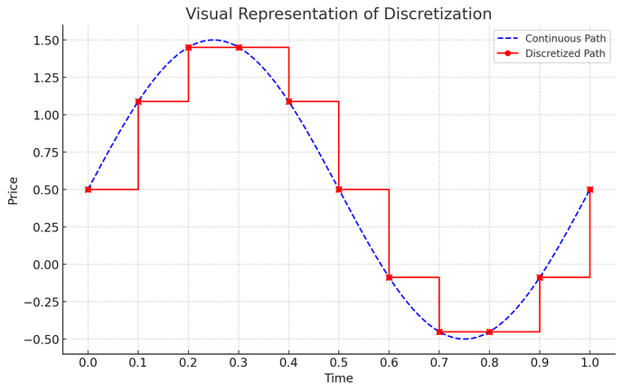
Many financial models, especially those dealing with derivatives pricing or risk management, are based on continuous-time processes like Brownian motion. Discretization helps in converting these continuous models into a form that can be numerically computed.

To simulate market dynamics for tasks such as option pricing, portfolio optimization, or risk assessment, continuous processes are discretized into discrete time steps. This allows for the application of numerical methods to simulate paths of asset prices, interest rates, or other financial variables over time.

Many models in finance, including the famous Black-Scholes model for option pricing, are based on differential equations. Discretization methods, like finite difference methods, are used to solve these equations numerically.

For risk management purposes, like Value at Risk (VaR) calculations, discretization helps in simulating the distribution of returns over a specific time horizon to assess the potential losses.

Discretization can also simplify complex models, making them more tractable and computationally feasible, although it might introduce some level of approximation error.

Now, let's take the example of pricing an exotic option using a discretization technique.

One common method for pricing these options is through Monte Carlo simulation, which heavily relies on discretization.

Example: Pricing a Barrier Option

A barrier option is a type of exotic option where the payoff depends on whether the underlying asset's price reaches a certain level (the barrier) during the option's life.

Assumptions:

• Underlying Asset: Stock with current price S0.
• Strike Price: K.
• Barrier Level: B (for a knock-out barrier option, the option becomes worthless if the asset price hits this level).
• Risk-Free Rate: r.
• Volatility of the Underlying: σ.
• Maturity: T years.
• Time Steps for Discretization: n (the total number of discrete time steps in the simulation).

Monte Carlo Simulation with Discretization:

• Discretize Time: Divide the option’s life into n small intervals, each of length Δt = T/n.
• Simulate Price Paths: For each simulated path (i.e., a possible future scenario for the stock price), use the geometric Brownian motion model to simulate the stock price at each time step. The formula for the stock price at each step is given by: S(t+Δt) = S(t) exp((r - σ^2/2) Δt + σ √Δt Z) where Z is a random variable from a standard normal distribution.

In each path, check if the stock price crosses the barrier level B at any time step. If it does, the option becomes worthless in the case of a knock-out barrier.

For paths where the barrier is not crossed, calculate the payoff at maturity, which could be, for example, max(S_T - K, 0) for a call option. Average the payoffs from all simulated paths and discount it back to the present value using the risk-free rate r.

 hashtag