
Suppose we are analyzing two stocks, Stock A and Stock B, for potential pairs trading opportunities. The first step involves examining the marginal distribution of each stock.
Through a detailed analysis, we find that Stock A follows a normal distribution with a mean return of 5% and a standard deviation of 2%. This marginal distribution provides insights into the expected returns and volatility of Stock A in isolation.
Stock B, on the other hand, has a marginal distribution that is skewed to the right, indicating that it has occasionally provided high returns, although its mean return is also around 5%.
Conditional Distributions
Now, we’re interested in understanding the behavior of Stock A given the performance of Stock B and vice versa. Let’s say on days when Stock B’s returns exceed its mean return of 5%, Stock A has a tendency to underperform, yielding returns below its mean. We calculate the conditional distribution of Stock A’s returns given Stock B’s performance exceeding its average returns.
When Stock B’s returns are expected to be above 5%, the trader might consider shorting Stock A, expecting it to underperform due to the observed conditional relationship.
The marginal distributions give the trader insights into the individual behavior of each stock, while the conditional distribution illuminates the interdependencies between the two stocks. For instance, if Stock B’s performance is exceeding expectations, the conditional distribution informs the trader about the likely underperformance of Stock A. Consequently, a pairs trading strategy could involve shorting Stock A and going long on Stock B during such scenarios.
A judicious integration of both distributions empowers traders to devise nuanced, data-driven pairs trading strategies, optimizing profitability while mitigating risks.
Copulas: Connecting Marginal and Joint Distributions
Copulas connect marginal distributions to joint distributions and reveal an advanced analysis landscape. In the realm of copulas, conditional probability functions play a pivotal role. Defined by the differentiation of the copula with respect to its parameters, these functions unveil nuanced insights into asset dependencies.
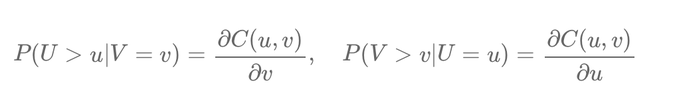
For instance, consider the conditional probabilities \( P(U > u | V = v) \) and \( P(V > v | U = u) \). These are calculated using the formulas:
\[ P(U > u | V = v) = \frac{\partial C(u, v)}{\partial v}, \quad P(V > v | U = u) = \frac{\partial C(u, v)}{\partial u} \]
Here:
- \( C(u, v) \): The copula function capturing the dependency between Stock A and Stock B.
- \( U \) and \( V \): The transformed uniform marginal distributions of the returns of Stock A and Stock B, respectively.
- \( u \) and \( v \): Specific values within these distributions.
For example, \( u = 0.7 \) represents the return of Stock A at the 70th percentile of its uniform distribution, and \( v = 0.8 \) represents the return of Stock B at the 80th percentile of its uniform distribution.
Application in Pairs Trading
Using copulas and conditional probabilities, traders can enhance pairs trading strategies by identifying and leveraging interdependencies between assets. For example:
- If Stock B is performing better than expected (above its mean), conditional probabilities from the copula might suggest a high likelihood of underperformance for Stock A. This insight supports a strategy of shorting Stock A and going long on Stock B.
- Copulas also help simulate joint movements of assets under different market scenarios, providing a robust framework for risk management.
By combining marginal distributions, copulas, and conditional distributions, traders can gain a comprehensive understanding of asset relationships, enabling more informed and precise trading strategies.
Écrire commentaire