In quantitative finance, understanding how changes in input variables impact outputs is essential for pricing, risk management, and portfolio optimization. Financial models often involve multiple
interdependent variables, making it crucial to analyze how small changes in one variable propagate through the system. One of the most versatile tools to capture such relationships is the
Jacobian matrix.
While commonly introduced in mathematics as a matrix of partial derivatives, the Jacobian matrix has broad applications across finance and economics. In finance, the Jacobian matrix is widely
used to measure sensitivities, transform risk metrics, and analyze multidimensional systems. It provides a framework to assess how complex relationships between variables evolve, helping
practitioners model dependencies across yield curves, asset prices, volatility surfaces, and credit spreads. By quantifying local changes and interactions, it plays a vital role in identifying
risks, valuing derivatives, and stress-testing financial models.
The Jacobian matrix is particularly valuable in situations where variables influence each other in non-linear ways. For example, it can be applied to calibrate yield curve models, estimate
implied volatilities, or map changes in option prices based on shifts in underlying asset values. Similarly, in portfolio management, it helps analyze how correlations and exposures interact,
providing insights into diversification and risk concentration.
This article introduces the core principles of the Jacobian matrix and illustrates its practical application using a fixed coupon bond sensitivity example.
The Jacobian Matrix: A Mathematical Tool for Transformation
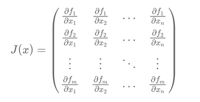
At its core, the Jacobian matrix generalizes the idea of derivatives to multiple variables. It measures how small changes in one set of inputs affect outputs. Mathematically, if we have a
function that maps an n-dimensional input vector to an m-dimensional output vector, the Jacobian captures the partial derivatives of each output with respect to each input. This is
expressed as a matrix:
In this matrix, each entry represents how one component of the output changes in response to a specific input. For instance, in finance, inputs might represent par rates1, while
outputs correspond to zero rates2 derived from them. The Jacobian then serves as a translation tool, quantifying how movements in par rates propagate through the yield curve to
impact zero rates.
Why the Jacobian Matters in Finance
Financial markets frequently rely on par rates because they are directly observable from bond prices. However, pricing models often use zero rates, which must be derived through bootstrapping3 from these par rates. This creates a challenge: how do we express sensitivities, such as PV014, in terms of market-observable par rates while preserving the mathematical rigor of calculations based on zero rates?
The Jacobian matrix resolves this problem. It allows us to convert sensitivities calculated with respect to zero rates into sensitivities relative to par rates. This transformation is particularly useful for hedging interest rate risks and aligning risk measures with market conventions.
A Practical Example: Bond Sensitivities
To illustrate the Jacobian matrix in action, let’s consider a fixed coupon bond. The bond’s price depends on zero rates, but its sensitivities are often expressed relative to par rates, which
traders and risk managers use. The relationship between the two is captured by the formula:
In this equation, \( PV01_{par} \) represents the sensitivity of the bond’s price to par rates, while \( PV01_{zero} \) measures its sensitivity to zero rates. The matrix \( J \) is the
Jacobian, which describes how changes in par rates affect zero rates.
To compute \( J \), we need to estimate how each zero rate responds to shifts in each par rate. For simplicity, suppose we have bonds with maturities of 1, 2, and 3 years, and their associated
par rates and zero rates are as follows:
To approximate the derivatives in the Jacobian matrix, we shift each par rate slightly (e.g., by 1 basis point or 0.0001) and recalculate the zero rates using bootstrapping. The derivative is then estimated as:
Computing this for each pair of zero and par rates produces the Jacobian matrix. For example:
Once the Jacobian matrix is established, we can transform sensitivities, making them easier to interpret and act upon in trading decisions.
The Jacobian matrix acts as a bridge between two different rate systems—zero rates and par rates—allowing us to translate sensitivities seamlessly. It combines mathematical precision with market
observability, enabling traders and risk managers to analyze and hedge interest rate risks effectively.
1 Par Rate: The par rate is the interest rate that equates the present value of a bond's cash flows to its par value. It represents the rate used to discount all future cash flows so that the bond's price equals 100 (par).
2 Zero Rate: The spot interest rate that discounts a single cash flow to its present value, assuming no intermediate payments. It represents the yield of a zero-coupon bond.
3. Bootstrapping: A method used to derive zero rates from market-observable par rates by solving iteratively for discount factors.
4. PV01: The price value of a 1 basis point (1/100th of a percent) change in interest rates. It measures the sensitivity of a bond’s price to small shifts in rates and is widely used in fixed-income risk management.🎓 Recommended Training: The Fundamentals of Quantitative Finance
Discover the essential concepts of quantitative finance, explore applied mathematical models, and learn how to use them for risk management and asset valuation.
Explore the Training


Écrire commentaire